Moving Averages are one of the oldest, simplest, and yet most powerful tools in the technical analyst’s toolkit.

This versatile TradeStation Moving Average indicator demonstrates the advanced functionality of our products, and is sure to become your go-to tool for all your moving average charting needs. A host of enhanced features include trend definition and rate of change. Like all our products, it comes accompanied with a full user manual detailing examples of trading strategies within which you can employ it.

TradeStation Moving Average Indicator Strategy Guide

Moving Averages have been around for a long time, and are a staple of technical analysis. Probably the most commonly used indicator, averages provide a simple and effective definition of a market’s trend, and are an integral component of countless other indicators, within which they often provide a smoothing function.

The Delphic Average has been color-coded to plot as a red or green line, providing traders with an instant visual confirmation of the slope of the indicator. We’ve also built in a variety of other convenient features so that you can get the chart analysis that you need, fast:

• Plot multiple averages from the same indicator. By changing the additional MA settings on the indicator’s ‘Inputs’ tab to a look-back period greater than zero, you can quickly plot several averages on your chart without having to add and format numerous analysis techniques.

• Switch to a different average type in just a few seconds. The averages plotted by the indicator can be changed from Simple to Exponential, Weighted, or Triangular, by entering ‘True’ in the indicator’s inputs tab by the average type you wish to display.

• Gauge the indicator’s trend objectively. The percentage change of a moving average – whether it is increasingly sloping or beginning to flat-line – is a simple but powerful method of measuring a trend’s momentum.

Switching the ‘PercentChange_On’ from ‘false’ to ‘true’ in the indicator’s inputs tab will cause the percentage change of the Delphic Average to be printed alongside the average (whatever the average type or length), so that you can easily make an informed assessment of the indicator’s movements. Subtle changes in momentum can provide a great heads up for scalpers.

In the rest of this document we reveal a number of trading strategies that make use of the Delphic Average, we examine performance reports for these setups in a variety of markets, and we discuss the pitfalls and limitations of lagging indicators and the dangers of over-optimisation and curve-fitting in system design. Whatever your timeframe or style, you’re bound to discover ideas here that will help you to make better use of averages in your trading.

Swing Trading with the ‘Halo’ Strategy

The following trading strategy has been developed from concepts presented by Larry Connors and Cesar Alvarez in the book ‘Short Term Trading Strategies that Work’.

If you want to work with daily price charts – a far less stressful and time-intensive style of trading than the rollercoaster ride of intraday scalping – but you aren’t sufficiently capitalised for a portfolio trend-following approach such as the one described later (or simply aren’t comfortable with the longer holding periods associated with trend-following), then a swing trading strategy such as the following may be a great place for you to begin.

Two Delphic Moving Averages are used, the first as a longer term trend filter, and the second to provide a profit target. Recognition of a simple chart pattern is also required: trades will be entered only when the market has made its highest high in three days (for short positions), or its lowest low in three days (for long positions).

A number of long entries are shown on the chart below (back-tests follow later in this article):

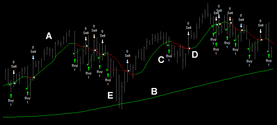
A The E-Mini S&P500 futures contract is trading above a 150-period Simple Moving Average.

B The SMA is colored green, indicating a stable upward trend.

C At point C we can see that price has made a new three day low (its low is the lowest of the last three days). The daily price bar has also closed below a 10-period SMA. A market buy order is entered at the close to establish a long position.

D A ‘Sell Limit’ order is placed at the profit target at the 10-period SMA. This will need to be adjusted on a daily basis after the close. This particular trade is exited for a small loss.

E Note that no stop-loss has been placed and that trade draw-downs can be significant, as at point E. The high percentage win rate of this strategy is offset by occasional large losses, and use of any kind of stop-loss will harm performance. If you are uncomfortable trading without a stop, place a very wide stop based on sound money management principles.

Indicator Overkill – The Pitfalls of Indicator Based Trading

Technical indicators do not provide some kind of magical shortcut that allows you to bypass the routines of careful study of price behaviour, and moving averages are no exception. Averages are a ‘lagging’ indicator; they take time to assimilate price action, and they tell you where price has been previously, not where it’s about to go.

To understand why moving averages lag, consider the example of the price histogram on the left below, in which the value of each bar represents the closing price for that period:

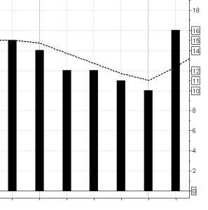We can calculate a moving average based on the closing price of each bar, over a three bar period. Starting from the third bar then, our 3-period moving average of the closing prices will be:

BAR 3 = (15 + 14 + 12) / 3 = 13.6
BAR 4 = (14 + 12 + 12) / 3 = 12.6
BAR 5 = (12 + 12 + 11) / 3 = 11.6
BAR 6 = (12 + 11 + 10) / 3 = 11

Now, what happens at the seventh bar? Our moving average will be calculated as follows:

BAR 7 = (11 + 10 + 16) / 3 = 12.3

With the moving average plotted on the price bars, it would look something like the right-hand chart above.

Suddenly our moving average line is pointing upwards in a bullish fashion and price has actually moved from closing below the average to substantially above it. Is this a buy signal? Unfortunately, we could only calculate this average on the close of the bar, or in other words once the move had already occurred. By the time we get a signal from our indicator (the moving average), price has already surged ahead. This is why price-based indicators are said to be lagging, and one of the reasons that we should be careful how we use them.

The longer the number of periods used by an indicator in its calculations, then the more the indicator will lag behind price action. If you imagine reducing the number of periods used to calculate a moving average of the closing price right down to a single period, then the indicator would no longer lag, but it would show nothing other than the closing price of each bar . . .

If the moving average now seems a little worthless, consider that even entering after price closes above the average we may still be at the start of a substantial rally. But before entering a trade we would surely want further confirmations of this. Was the breakout on high volume, for example? Was it in line with the longer term trend? Is the market already overbought?

Most indicators work well in trending markets, but come unstuck in sideways ranges. Using nothing but a crossover of two moving averages, you can easily catch great, profitable moves when a market trends. But unfortunately you may well give most or all of these profits back if you continue to follow this system when the trend ends and the market moves sideways. No sooner will your moving averages give an entry signal than the market will have changed direction against you. Unfortunately, you would not only need to be able to recognise when such a period has commenced in order to stop trading your indicator based system, but you would also need to know when it had ended, otherwise you wouldn’t be in at the start of the next profitable trending leg.

The following chart shows the application of a very simple intraday trend-following strategy, in which the market is bought whenever a 4SMA crosses above a 12SMA, and sold when it crosses below:

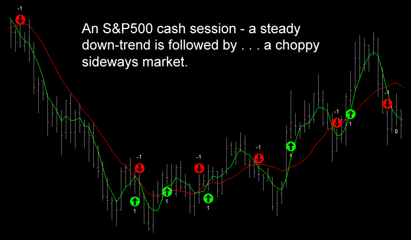
A total of eleven trading signals were generated in the S&P cash session shown:

Trade Number	Position	Dollar Profit
1	Short	$525
2	Long	-$50
3	Short	-$62.50
4	Long	-$25
5	Short	-$50
6	Long	-$12.50
7	Short	-$200
8	Long	-$62.50
9	Short	-$187.50
10	Long	-$150
11	Short	-$75

Total Net Profit: -$350

Trading this strategy, you would start out your day with a welcome $525 profit on the first trade, but in the subsequent trades you would lose a grand total of $875 points. Bear in mind that we haven’t even factored in slippage or commissions here – one of the problems with this type of system is that it causes you to overtrade enormously. In fact, you’re always in the market, either long or short.

So how would this strategy perform over a two year period if we deduct commissions? You can probably already guess the answer:

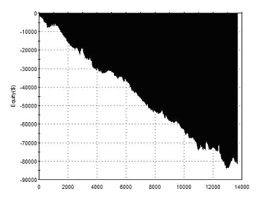	Total Net Profit Profit Factor Long Profit Factor Short Profit Factor Total Trades Percent Profitable Avg Trade Net Profit Maximum Drawdown	-$81,465 0.86 0.88 0.85 13,678 31.91% -$5.96 -$83,945
Performance Report – Moving Average Crossover – @ES

As you can see above, the strategy produces a net loss over a sustained period and over thirteen thousand trades. The downward slope of the equity curve is remarkably smooth, suggesting that doing the exact opposite and buying on a negative crossover would actually be a profitable strategy.

To trade profitably with averages, or any other lagging indicator, you really need to bring your own perspective of the nature of price behaviour into the equation. It is often said that “you can’t trade the market – you can only trade your beliefs about the market”. You should be able to encapsulate your beliefs about the markets in a very simple statement, such as one of the following:

• Prices tend to revert to their mean average price over time.
• The stronger moves are always in the direction of the long term trend.
• Although price may remain range-bound at times, ultimately there will always be sustained trends in the market.
• A trend is more likely to continue than to reverse.
• Long term success will always ultimately depend on a few positive outliers.
• Recognising value is the most important element to understanding what stocks to buy.

Only once you are in possession of a model for price behaviour in your chosen market(s) that you truly believe will you be able to make full and appropriate use of technical tools such as moving averages, and trade confidently with them to achieve your profit goals.

In the ‘Luxor’ MA crossover and pattern recognition strategy that follows, we will look at ways to try and pick out winning signals like the first crossover in the example above, and avoid too many whipsaw signals like those that followed.

The Principles of Trend-Following

Simple strategies for exploiting sustained price trends are as old as the markets are, and they continue to be used widely by the large capital management firms and hedge funds. The aim with this type of approach is not to pick tops and bottoms, but to profit from the ‘middle’ of the trend.

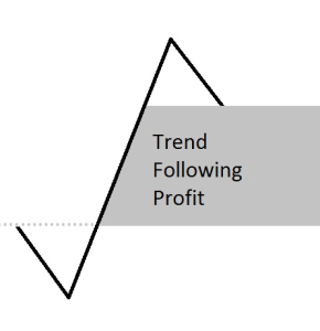
Take a look at both the simplified diagram and the real price chart below, which show the portion of a trend from which this type of strategy aims to profit:

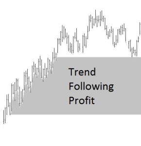As you can see, this strategy means waiting until a trend is clearly established before entering the market and waiting until it is decidedly ended before exiting. This has two consequences that many traders find difficult to accept:

• It is instinctive to ‘buy low and sell high’, but the trend-follower does the opposite – they buy a market when it is making new highs. This is because they aim to profit when the market continues to make new highs after their entry, and a long term trend is established.

• Trend followers never exit at the optimal point; they allow the trend to reverse and give back some of their profits to the market before exiting. It is only by allowing this reversal to occur that they can be sure the trend from which they have profited is over.

Another issue is that, during periods when there are no sustained trends, trend-following systems tend to accumulate small losses, sometimes resulting in significant draw-downs of the equity curve. One way to minimize the impact of draw-downs is to trade the strategy across a portfolio of markets. Modern Portfolio Theory suggests that these markets should be as uncorrelated as possible: the idea is that when a draw-down is being experienced in one market, another will be trending, thereby off-setting losses and smoothing the equity curve. It is not uncommon for large trend-following funds to take positions in several hundred instruments . . . but then they are exceptionally well capitalised compared to the average trader.

A diversified ten market portfolio such as might be feasible for a private investor with a capital base of $100,000 could look something like the following:

METALS:	Gold	ENERGIES:	Crude Oil
GRAINS:	Soybeans	INTEREST RATES:	5 Year Note
SOFTS:	Cotton		Euro Bund
CURRENCIES:	British Pound	STOCK INDICES:	S&P500
	Japanese Yen		Nikkei 225

For more detailed discussion of these and other trend-following topics, we recommend Curtis Faith’s ‘Way of the Turtle’, and Mike Covel’s ‘Trend Following’.

Trend Following with the ‘Luxor’ Entry Strategy

The approach described below was inspired by the ‘Luxor’ strategy described in Emilio Tomasini and Urbane Jaekle’s book ‘Trading Systems’, itself based upon early TradeStation development forum articles. This strategy combines a simple moving average crossover with basic pattern recognition, the idea being that we enter a market only when price bar action displays a show of strength or weakness.

Criteria for Long Entries:

• The Fast Moving Average is above the Slow Moving Average.
• The Fast Moving Average is upward sloping (ie colored green).
• Today’s close is greater than yesterday’s high.

Criteria for Long Exits:

• The Fast Moving Average crosses below the Slow Moving Average.

The Slow Moving Average is a 250-period SMA. The Fast Moving Average is an SMA Average with a number of look-back periods that has been optimised (to the nearest 10 periods) over the prior ten years of data (yearly re-optimisation should be undertaken). For short positions the entry and exit criteria are reversed.

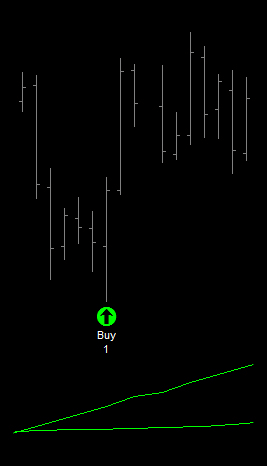
The Chart below shows a long entry in the British Pound futures contract. The optimal Fast Moving Average for this market is currently 170-periods. At point A the 170-period DELPHIC Average crosses above the 250-period average (signalling the exit for an unprofitable short position).

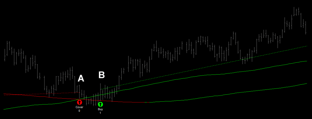
Nine days later, at Point B, the daily close is greater than the prior day’s high, and a long position is established. Note that because the exit criteria are less stringent than the entry criteria, there will be periods like the nine days above, when the system is flat the market.

The Perils of Over-Optimisation and Curve-Fitting

One of the very real dangers when backtesting a strategy is ‘over-optimisation’ or ‘curve-fitting’. By manipulating the parameters of numerous inputs such as moving averages, we can find a metric that would have been hugely profitable for pretty much any market. But this is trading with the benefit of hindsight; curve-fitted strategies look great when applied to historical data, but their real-time performance is invariably atrocious.

Does this mean that optimisation is to be avoided? No. It’s pretty much unavoidable, in fact. You can choose a completely random set of parameters, but they might just happen to be those that would have performed well historically, giving you a false sense of the effectiveness of a system.

Whenever you choose to trade a particular market, timeframe, or indicator, you run the risk of over-optimisation or ‘curve fitting’. But not to optimise at all is dangerous, a paradox that is succinctly described Eckhardt in ‘New Market Wizards’:

One widely recognised way to reduce the probability of curve-fitting is to limit the number of parameters that are optimised (what Eckhardt calls ‘degrees of freedom’).

In the strategy above we took an extreme approach, optimising only the fast moving average, and hence we expect the strategy would be reasonably robust in real-time trading. Even so, an intuitive element of optimisation doubtless crept in when we selected 250 periods as a global parameter for the slow moving average . . . although it is probably not the absolute optimum solution, it is one that we know from experience would likely have performed well historically. When it comes to optimisation there are pitfalls at every step of the way!

Another telltale sign of over-optimisation is when a particular parameter produces highly profitable results (A 60 period MA, for example), but its immediate neighbours do not (so that a 50 or a 70 period MA loses money).

In real-time trading you are more likely to end up with the performance of one of those neighbouring parameters, so they need to be good.

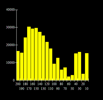From the chart on the right we can see that the most profitable length for the moving average was 170 periods. But look at how poorly a 180 period average performed by comparison . . . The wisest choice here going forwards might be the 150 period moving average.

The 150 period moving average is positioned in the centre of a block of similarly profitable values. The results of trading with any of these neighbouring values would be acceptable to us.

As a rule, we want to choose a parameter that is situated in a block of virtually equally profitable parameters – this will greatly increase the probability that our strategy will perform almost as well in the future as it would have in the past.

The ‘Luxor’ entry strategy above is really given as a point of inspiration for those fortunate enough to have considerable risk capital to work with. Though trend-following undoubtedly still works (see the results of Bill Dunn, Liz Cherval, or John W Henry, to name but a few), the simple breakout strategies that made millionaires of Richard Dennis and his ‘Turtles’ in the 1980s would soon empty your account nowadays.

Dennis’s partner, William Eckhardt, continues to manage a successful multi-billion dollar trend-following fund to this day, but he most certainly does not do this by buying twenty-day breakouts – you’re going to need something a little more sophisticated to survive as a trend-follower in today’s markets . . .

Art Collins’ ‘Four Rules of Prudent Optimisation’ RULE 1: Make sure your best outcome resides in the neighbourhood of similarly good numbers. You don’t want to act off a standout diamond in the rough. RULE 2: System Results should hold up in other markets, especially those closely related to your original testing field. RULE 3: Profits and losses should be dispersed somewhat evenly throughout your data field. RULE 4: Understand your drivers. Test only in support of theories or concepts about the markets that you believe to be true. “Every time I need to use an equal to, greater than, or less than sign I am, in fact, formulating a rule. For me, the trick is to keep all these signs down to a minimum, preferably below five for the entire strategy. As you will discover, if you are being honest about what constitutes a sign, it is very difficult.” Thomas Stridsman – Trading Systems that Work

Testing the ‘Halo’ Strategy. . .

Because the ‘Halo’ strategy (detailed earlier in this article) enters the market counter to the short term (three day) trend, we would typically expect it to perform better in markets that have a stronger propensity to revert to the mean in the longer term.

The S&P500 used in the example above is certainly one market where this has been the case historically (around 70% of all ES trading sessions revisit their prior day’s average price), and this pronounced centralising tendency is echoed across most other major international indices (eg. Dax, Nikkei, FTSE, Nasdaq, Russell, DJIA).

In the book ‘High Probability ETF Trading’, Larry Connors and Cesar Alvarez suggest that Exchange Traded Funds in general exhibit a more pronounced centralising tendency. We have therefore chosen to conduct the back-tests of this strategy across a number of ETFs, which allow participation across a diverse range of international markets including commodities, sectors, interest rate, and stock indices.

The net profit and the profit factor are shown for each ETF are shown below.

The performance reports below use a 75-period moving average filter across all markets. A fixed trade size of 1,000 shares was used. No slippage or commissions were deducted.

Symbol	Name	Net Profit	Profit Factor
DIA	Diamonds Trust (ETF)	$35,980	1.43
EEM	iShares MSCI Emerging Markets (ETF)	$45,810	2.17
EFA	iShares MSCI EAFE Index (ETF)	$30,710	1.52
USO	United States Oil Fund (ETF)	$44,660	2.06
EWH	iShares MSCI Hong Kong Index (ETF)	$10,690	1.73
EWJ	iShares MSCI Japan Index (ETF)	$7,760	1.67
EWT	iShares MSCI Taiwan Index (ETF)	$9,100	1.53
EWZ	iShares MSCI Brazil Index (ETF)	$50,010	1.73
BND	Vanguard Total Bond Market (ETF)	$10,060	3.57
FXI	iShares FTSE/Xinhua China 25 Index (ETF)	$30,820	1.70
GLD	SPDR Gold Trust (ETF)	$13,420	1.18
ILF	iShares S&P Latin 40 Index (ETF)	$35,010	1.81
IWM	iShares Russell 2000 Index (ETF)	$59,590	2.24
IYR	iShares Dow Jones U.S. Real Estate (ETF)	$65,850	2.46
QQQ	PowerShares QQQ Trust (ETF)	$17,930	1.40
SPY	SPDR S&P500 (ETF)	$84,320	2.38
XHB	SPDR S&P Homebuilders (ETF)	$6,270	1.24
XLB	Materials SPDR (ETF)	$20,780	1.63
XLF	Financial Select SPDR (ETF)	$22,630	2.47
XLI	Industrial SPDR (ETF)	$20,540	2.25
XLV	Health Care Select SPDR (ETF)	$16,820	1.75

Although the net performance here seems excellent considering we have not optimised our parameter for either individual markets or portfolio performance, it should be noted that the results above do not include any measure of the volatility of return over the test period. In other words, there is no information about the draw-downs required to achieve these results. Along with further detailed testing, a thorough understanding of Modern Portfolio Theory would be an essential next step here.

Many of these ETFs correspond in an obvious way to a retail futures contract (the DIA and the Mini Dow futures YM contract, for example), and where this is the case we cannot detect any evidence of a substantial difference in the performance of the strategy between the two. The test below shows the results trading a single E-mini S&P500 futures contract, equivalent to the SPY:

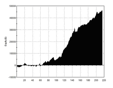	Total Net Profit Profit Factor Long Profit Factor Short Profit Factor Total Trades Percent Profitable Avg Trade Net Profit Maximum Drawdown	$46,040 2.66 3.03 2.37 215 83.72% $214.14 $6,125
Performance Report – ‘Halo’ Strategy – @ES – Daily Bars – 06/05/2010-06/05/2012

One of the advantages of trading ETFs, it should be noted, is that they are not heavily leveraged, meaning that it can be easier to control risk and grow a small account. ETFs can be more difficult to short than futures, however, and are often less liquid.

// TradeStation EasyLanguage Strategy Code // Swing Trading ‘Halo’ Strategy for Daily Bars Inputs: Length(75), Trgt(10); If Close<Average(Close,Length) and Average(Close,Length)<Average(Close,Length)[1] and Close>Average(C,Trgt) and High=Highest(High,3) then Sellshort this bar; Buy to cover next bar at Average(Close,Trgt) limit; If Close>Average(Close,Length) and Average(Close,Length)>Average(Close,Length)[1] and Close<Average(Close,Trgt) and Low=Lowest(Low,3) then Buy this bar; Sell next bar at Average(Close,Trgt) limit;

 

Advanced Moving Average Platform Requirements: TradeStation 10.0 Support Documents: Indicator Guide Moving Averages are one of the oldest, simplest, and most powerfully versatile tools in the technical analyst’s toolkit. This indicator demonstrates the advanced functionality of our products. Download this indicator for free: Email(required) Submit