Decades before computers and algorithmic trading dominated the financial markets to the extent that they do today, floor-traders would to take nothing more than a pencil and paper into the pits of the Chicago exchanges with them, and they would calculate a simple series of price levels before the opening bell.
Pivot Levels are now very widely used by off-floor traders.
So what’s so special about the Delphic TradeStation Pivot Points indicator? In terms of their calculation, the pivots are pretty much standard, but they’ve been designed to be convenient to set up, visually customisable and easy to interpret and, most importantly they come with a user manual packed full of smart strategies to enable you to take full advantage of the daily opportunities that these levels present.
Here are some of the features of this indicator:
Intermediate Pivot Levels
Following large range days that produce highly spaced pivots, it is common practice to plot the ‘mid’ level between each two standard pivots. With the Delphic Tradestation Pivot Points you can switch this option on, and you can specify how many points apart the standard pivots must be before a mid level will plot.
Confluence Zones
The Delphic Pivots can be directed to search for confluences with other price chart indicators. When these are discovered – both the daily pivot and a 200-period moving average in close proximity, say – then a broader grey zone will be plotted around the pivot.
Daily Pivot Trend
One of two ‘trend’ functions, this study paints bars green when the day’s pivot is higher that that of the preceding day. This is like using a very fast moving average on a daily chart to gain an intraday bias, but rather than using the closing price alone, this average combines the high, low, and close. This function can be switched on by entering ‘1’ under ‘DailyTrend_On’ in the indicator’s ‘Inputs’ tab.
Intraday Pivot Trend
This second paint bar study colours bars according to the intraday trend. This is considered to be up (green) if the highest intraday high is further from the daily pivot than the lowest intraday low is below it (and visa-versa for down trends). Far less choppy than other trend indicators, this can be a useful filter for intraday trading strategies. Enter ‘1’ under ‘IntradayTrend_On’ on the indicator’s Inputs’ tab to activate.
Audio Alerts
Switch on the indicator’s audio alerts, and you’ll be alerted every time price approaches a pivot level, so you can focus your analysis elsewhere in the meantime.
User Defined Colours and Labelling
The colours of the pivot levels can be adjusted, and each pivot is clearly labelled to the left of the chart, making the Delphic Pivot Points visually clearly and easy to work with.
Adjusting the Indicator’s Inputs in TradeStation
To change any of the Delphic Pivot Points indicator settings, simply right click anywhere on the indicator after adding it to your chart, then select the ‘Format Delphic Pivots’ option from the menu. On the ‘Inputs’ tab at the top of the pop-up box, you’ll find a list of every adjustable parameter for the indicator. The table below shows each parameter along with a description of how it can be changed.
| Name | Value | Description |
| MidPivots_On | False | Entering ‘True’ will turn on the intermediate pivot levels. |
| PivotSeperation | 0 | Specifies required Pivot spacing for MidPivots to be plotted. |
| DailyTrend_On | False | Entering ‘True’ will turn on the Daily Trend function. |
| IntradayTrend_On | False | Entering ‘True’ will turn on the Intraday Trend function. |
| Indicator | 0 | EasyLanguage code highlights confluences with pivots. |
| ResistanceColor | Red | Select a color for R1, R2, R3 and intermediate pivot levels. |
| SupportColor | Green | Select a color for S1, S2, S3 and intermediate pivot levels. |
| PivotColor | White | Select a color for the Daily Pivot level. |
The Delphic Pivot Point Formulas
Pivot = ( PriorHigh + PriorLow + PriorClose ) / 3
R1 = ( Pivot * 2 ) – PriorLow
S1 = ( Pivot * 2 ) – PriorHigh
R2 = ( Pivot + PriorHigh ) – PriorLow
S2 = ( Pivot – PriorHigh ) + PriorLow
R3 = ( R2 + PriorHigh ) – PriorLow
S3 = ( S2 – PriorHigh ) + PriorLow
The Pivot Pairs Strategy
Statistical Arbitrage, often referred to as ‘Stat Arb’, was one of the mainstays of early quantitative trading, when emerging hedge funds such as Citadel and Process Driven Trading would automate execution across vast, constantly shifting portfolios of stocks and other derivatives. The following description is taken from Scott Patterson’s ‘The Quants’:
“Gerry Bamberger discovered stat arb almost by accident. Bamberger wrote software for Morgan’s block trading desk, which shuffled blocks of ten thousand or more shares at a time for institutional clients such as mutual funds. The block traders used a “pairs strategy” to minimize losses. If the desk held a block of General Motors stock, it would sell short a chunk of Ford that would pay off if GM took a hit.
Bamberger noticed that large block trades would often cause the price of a stock to move significantly. The price of the other stock in the pair, meanwhile, barely moved. This pushed the typical gap between the pairs, the “spread”, temporarily out of whack. Suppose GM typically traded for $10 and Ford for $5. A large buy order for GM could cause the price to rise temporarily to $10.50. Ford, meanwhile, stayed at $5. The “spread” between the two stocks had widened.
Bamberger realised he could take advantage of these temporary blips. He could short a stock that had moved upward in relation to its pair, profiting when the stocks returned to their original spread. He could also take a long position in the stock that hadn’t moved, which would protect him in case the other stock failed to shift back to its original price – if the historical spread remained, the long position would eventually rise.”
The following strategy is a very basic version of the statistical arbitrage concept, in which the daily pivot will be used to identify trading opportunities. When the instruments in a short-term correlated pair each diverge to opposing sides of their daily pivot, we short the contract that opens above its pivot, and we buy the contract that opens below, on the assumption that the spread between the two will diminish during the next day’s trading.
The process we will undertake is as follows:
Identify a Suitable Pair for Trading.
Normally something like the Dickey-Fuller test would be used to identify co-integrated pairs, but we are only concerned with a very short (one day) time horizon, so we can just look for pairs where the 1-Period Correlation Coefficient is typically 1. It is usually best to start with pairs which we can expect to be correlated for obvious fundamental reasons; for instance, two indices such as the S&P500 and the NASDAQ which are both representative of sentiment towards US companies and share some constituent stocks. In the case of the futures contracts pertaining to the markets above, the ES and the NQ, the single period correlation coefficient has been 1 on 84 percent of trading days over the past ten years. In other words, they usually both close in the same direction, whether that be up or down. Of the 399 days when their closes have diverged, on only 60 occasions (13%) did the direction of their close continue to diverge on the following day.
Calculate Relative Position Sizes.
The basic aim with this step is to ensure that we are trading dollar equivalent amounts of each contract. We start by multiplying each contract’s current price by it’s point value, for example:
@ES = 1309 x 50 = $65,450
@NQ = 2483 x 20 = $49,660
These dollar amounts tell us how much one contract of each is worth. We can now calculate a simple ratio, using one contract as the base for the pair (exactly as with spot forex prices). We’ll use the ES as our basis:
65450 / 49660 = 1.318
In other words, for each ES contract that we trade, we will need to trade 1.318 contracts of NQ. This isn’t possible, but we can multiply using this ratio so that we would trade 13 contracts of NQ for every 10 contracts of ES. This ratio will need to be re-calculated on a daily basis.
Calculate the Daily Pivot for Each Instrument.
When one of our instruments closes above its daily pivot and the other closes below, we short the former and buy the latter on the following open, sizing our position in each according to the formula above. Note that we’re using 24hr charts here, so there should be little difference between close and subsequent open prices. All positions are exited after one day.
To see how this performs we need to combine the equity curves for each instrument. With the TradeStation platform this can be done either by using a 3rd party portfolio analysis app, or by shipping the data out to excel manually as I have done here.
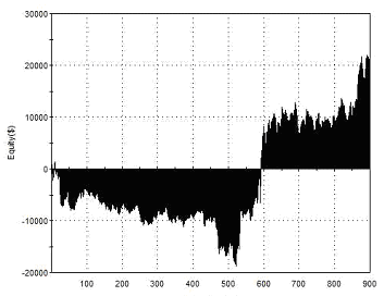
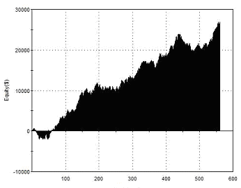
Here is the equity curve for this strategy, using 10 ES contracts as the base unit:
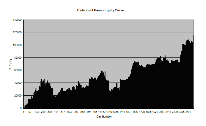
Although the results are clearly fairly positive here, there are a few things to note:
- Firstly, the draw-downs are significant, although they are representative of a full 10 contracts and are as low as $4000 per individual contract.
- Secondly, the strategy concludes with a net profit of $116,035 after 329 trades, meaning the average profit per trade is $352.68. Remembering that we’re trading 10 contracts of the base unit here, then that equates to an average trade profit of $35.20 per ES contract.
One thing that we haven’t done is subtract any execution costs from our results. Fortunately, doing so needn’t have any great impact on the equity curve we see above: entering using a limit order at the prior day’s close works just as well. In fact, it slightly improves performance with an average trade profit of $400.10.
As you’re never likely to exit on the closing tick exactly, the effects of your exit are unlikely to make too much difference either – sometimes you’ll see a few ticks improvement and sometimes a few ticks degradation.
Improving the Pivot Pairs Strategy
One useful filter to consider might be the introduction of a rule stating how far each instrument must close above or below its pivot in order for a position to be established on the following open.
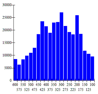
The tests below aim to do this, though for simplicity this rule has been applied only to the NQ data, with the number of points shown along the x-axis:
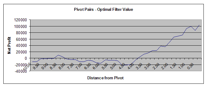
Looking at the net profit alone is not telling us much here – although the strategy is not profitable when the distance from the Daily Pivot is greater than 3.75 NQ ticks, doing so produced very few trades compared to entering when the distance was a single tick, making the data sample far from robust. The increased profits are possibly just the result of higher trading frequency.
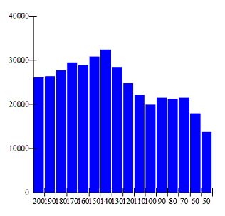
If we take a look at the average profit per trade, this should be more meaningful, although we must also bear in mind that data to the left of this graph is derived from a very small sample size:
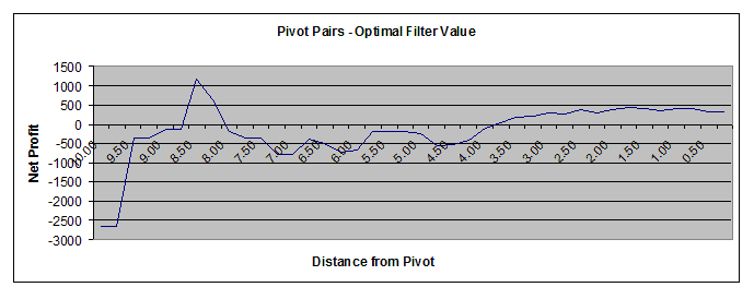
This seems to confirm our suspicions: although net profits improve when we reduce the distance from the pivot required for entry, the average profit per trade remains roughly the same. The point at which both these graphs cross below the x-axis appears to provide a more meaningful filter: it makes sense to establish a position only when the NQ closes within 3 points of its pivot. At greater distances the expectation of a profitable outcome is negative for the one day time exit we’re using here.
Earlier we discussed the average profit per trade relative to the costs associated with entering and exiting a position. Often when this issue arises it can make sense to move to a higher timeframe to trade the method in the hope that the average profit will increase while the costs of trading remain the same.
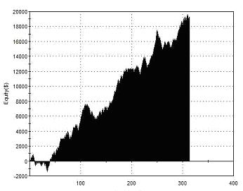
So finally, let’s take a quick look to see what happens when we apply the basic strategy using weekly charts and weekly pivots:
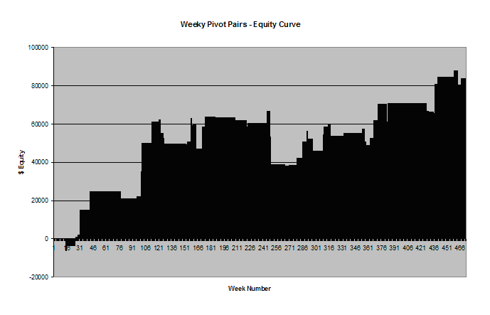
Strangely, the main contributor to our net profit is now the ES rather than the NQ, but this is somewhat immaterial as we’re not making any attempt to predict which side of the pair will profit in any given scenario. Most importantly, our net profit is $83,690, or $141.84 per contract per trade. This would very comfortably overcome costs.
Here are some more ideas for developing this strategy further:
- Holding 10 contracts for weeks at a time requires considerable margin. One way around this would be to substitute the appropriate ETFs for the futures contracts, de-leveraging the strategy and permitting share based position sizing.
- Determine whether closes at greater distances from the pivot have a greater likelihood of a profitable outcome if we increase the time window before exiting the position to more than one day.
- Study the relationship between volume and signal quality – are divergences in the pair more likely to revert when they occur on higher or lower relative volume?
John Carter’s Pivot Strategy
The following technique is described in detail by John Carter in his book ‘Mastering the Trade’. Essentially, Carter waits for a strong up-trend to develop that ‘violates’, or trades cleanly through, an overhead pivot level. The aim is then to buy a pullback to this violated pivot level using a limit order. Rules are reversed for short entries.
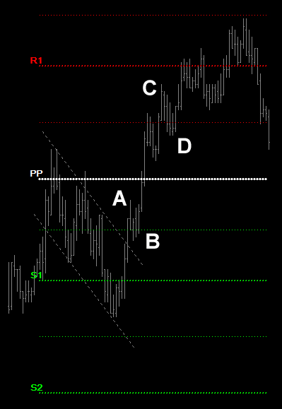 |
Rules for Long EntriesA The E-Mini S&P has been in a strong uptrend pre-market. A few hours into the cash session, at point A, it breaks out from a bullish flag formation and trades well above the S1 Mid Pivot. B At this stage a ‘Buy Limit’ order is entered a tick above the S1 Mid Pivot. As the market pulls back briefly, the buy order is filled at point B. C Profits can be taken with a target at the next pivot level, or via a trailing stop. At point C the process is repeated, as a strongly trending market pushes through the R1 Mid pivot. D A limit order placed at the pivot will establish a long position as the market pulls back at point D. Note that a further profitable buying opportunity occurred at the R1 Pivot level, though by this time you might have been wondering whether the move wasn’t overextended. |
| The chart above demonstrates an idealised scenario. This type of strategy typically works well in strongly trending markets, but identifying such markets at an early stage is no easy feat. And markets that move with real momentum often never pull back far enough to fill limit orders.
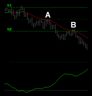
You might like to consider combining the pivots with another momentum strategy, such as the LBR ‘Grail’ setup, incorporating an EMA and the ADX in order to improve the probabilities of success. The chart on the right shows two examples of shorting opportunities combining these two strategies at A and B. With the ADX showing a strong trend, pullbacks to the EMA and a pivot provide short entries. |
 |
Scalping with Limit Orders – Professional Execution Techniques
There is a fine line between successful and unsuccessful limit order scalping, and it has almost nothing to do with entries or exits, and everything to do with smart order execution.
Many strategies appear profitable when back-testing software is instructed to assume a fill when price trades at the limit, but the reality is that up to a third of all such orders would not be filled. What’s worse, all the losing trades would still be filled (as by definition they must trade through the limit). The only way to guarantee that a fill would have occurred when back-testing is to include only those limit orders where price traded through the limit. Do this and many promising limit order strategies fall apart . . .
Fortunately the strategy above does not, but its profitability is still reduced. So is there anything that you can do to improve your chances of a limit order fill?
Level the Playing Field – Trade Futures
Stocks, ETFs, Spot Forex, and many other markets have Market Makers, Liquidity Providers, and Floor Traders, all of who are allowed to jump to the front of the queue and get their limit orders filled before yours. However, the order books of the electronically traded futures contracts operate on a ‘FIFO’ (first in, first out) basis. That means that if your limit order hits the exchange servers before JP Morgan’s order does, you get filled first!
Don’t Place Orders, Un-place Them!
Most of the major market players use highly sophisticated algorithmic trading solutions to submit their orders. Rather than placing orders at a particular level once an entry signal is generated, they simply pepper the order books at multiple levels and then cancel the orders that are not required as price approaches those levels. The orders that they leave for execution have consequently been sitting there for a long time and are near the front of the queue.
This is difficult to do this with many strategies, but because the strategy above uses a leading, predictive indicator, rather than a lagging one, you can submit your orders pre-market. Get your limit orders in as soon as the market opens, or preferably before, and you should be jostling at the front of the order queue alongside the HFT firms.
Front-Run . . . Then Front-Run Some More . . .
To increase your chances of being near the front of the queue, you want your limit order to join the shortest queue possible. This isn’t going to happen at a pivot – there are thousands of retail orders queuing there. Place your order in front of these levels (below a pivot for a sell limit, and above for a buy limit), and the chances of a fill are greatly improved. If you’re familiar with reading the order book you can place multiple orders around a pivot pre-market to try and get to the head of the queue and then, as price approaches, decide which order is most likely to be executed based upon the depth of the market.
Drive A Hard Bargain
Most brokerage software includes a function that causes limit orders to be converted to market orders after a certain time period has elapsed. You need to disable this function. You need to get a fill at your limit order price or better, not have a commission-hungry execution platform start chasing the market and paying up for the spread (or worse). So drive a hard bargain, and always buy at the bid and sell at the ask.
| Some Dos and Don’ts of Pivot Trading | |
| DO think of levels as ‘price areas where something may happen’, rather than as guaranteed support or resistance. Whether price either respects or ignores these levels is significant, and tells you something about the market’s behaviour. | DON’T be tempted by the lure of more extravagant pivot point formulas. Stick with the standard, age-old calculation – this is what the vast majority of traders use, and it is the herd behaviour of these traders that you can exploit. |
| DO employ a pivot strategy that is appropriate to the type of market that you are trading. | DON’T use pivots calculated from anything other than the cash session high, low, open, and close. |
| DO remember to adjust the session time inputs when the previous session’s close was different to the usual session (for example when exchanges close early for holidays) | DON’T use pivots in the forex markets. Pivots are only used in these markets by retail traders, and the huge depth of inter-bank liquidity swamps their effect. |
The Indicator’s Confluence Function
The next technique uses one of the enhanced features of the Delphic Pivot Points to look for confluences of support and resistance alongside a secondary indicator.
It is up to you to determine what the second indicator will be, so for those who are not familiar with TradeStation’s programming language, the following reference is provided. Once you’ve entered one of the following indicator descriptions in the Delphic Pivot Points ‘Inputs’ tab, if the secondary indicator lies in any close proximity to a Pivot level, then that Pivot will be highlighted with a thicker grey line.
| // TradeStation EasyLanguage Code for Pivot Indicator Inputs
Average(Price,Length) // e.g. Average(Close,20) for a twenty-period simple moving average of the closing price. XAverage(Price,Length) // e.g. XAverage(High,4) for a four-period exponential average of the high price of each bar. Highest(Price,Length) // e.g Highest(High,20) will give the upper band of a Donchian Channel, as used in the famous Turtle’s four-week breakout rule. For the lower band use Lowest(Low,20). Average(Price,Length)+(NumberofDeviations*StandardDev(Price,Length,DataType)) // e.g. Average(Close,20)+(2*(StandardDev(Close,20,1)) would give the upper Bollinger Band with the standard twenty-period settings. Note that ‘DataType’ should always be entered as ‘1’. For the lower band, the addition should be a subtraction: Average(Close,20)-(2*(StandardDev(Close,20,1)). |
Confluences Of Support and Resistance Pivot Strategy
In this approach we use the secondary indicator feature of the Delphic Pivot Points to identify areas where we can expect to find support from both a Lower Bollinger Band and a Pivot Level within a longer term uptrend, or resistance from an Upper Bollinger Band and a Pivot Level within a downtrend.
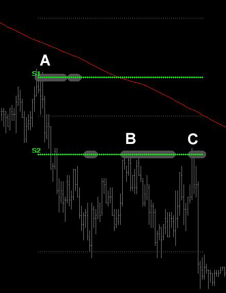
On a 5 minute chart, a 200-period simple moving average has been added. We can see the price is bearish and has been trading below this average. The Delphic Pivot Points have been added, and the code for the Upper Bollinger Band is entered on the indicator’s ‘Inputs’ tab:
Average(Close,20)+(2*StandardDev(Close,20,1))
Rules for Short EntriesA At point A you can see that the Upper Bollinger Band and the S1 level must lie in close proximity because this Pivot has been highlighted in grey. A ‘Sell Limit’ order is entered at this level and this would be filled within minutes of the open. B At point B a further opportunity to short rallies to S2 occur. C This repeats again at point C with a second failed rally to S2. This method works best when a tighter stop loss is used and the profit target is many multiples of the initial risk. Stop-losses can also be trailed to nearby Pivots and Intermediate Pivots to lock in profits. You might wish to experiment with a different trend filter to the moving average used in this example, or to employ tape-reading methods to assess interest as a price approaches a pivot. |
 |
Pro-Trader TipsPRO TIP: Analysis of volume is an essential part of John Carter’s pivot strategy. Volume is used to decide whether a day has trend potential, or will be ‘choppy’. If the volume after 10am on a 5 minute chart of the ES is consistently under 10,000 contracts per bar, then expect a choppy, narrow range day. If it remains above this the market should produce powerful and volatile price movements. Ignore the volume of the markets in the first half hour of trading when many queued orders are executed. PRO TIP: Trend or no trend? Fund manager Tony Crabel noted in ‘Day-trading with Short Term Price Patterns’ that strong trending days often follow narrow range, low volatility days. Crabel places special emphasis on NR7 days, when the range is the narrowest of the prior seven days, as well as inside days, or ‘harami’ candles. “In the long run it will be the management of the trade after the entry that counts more than the initial entry point” Linda Bradford-Raschke |
The Daily Pivot as a Swing Trading Tool
As you will have gathered if you have read through the calculation for the daily pivot above, there is nothing very complicated or ‘magical’ about this number, it’s simply an average of the prior day’s high, low, and closing price.
Rather like a volume-weighted average price, the daily pivot should give us an approximate idea of perceived value during the prior cash session, reflecting the extent to which buyers were able to drive prices higher and sellers were able to drive prices lower, along with who was in control by the end of the day.
The following strategy uses the daily pivot calculation as a ‘price proxy’, or estimation of the underlying value, of the e-mini S&P futures contract (@ES), to identify short term entries into longer term trends. The basic entry concept is very simple and is as follows:
When today’s pivot is lower than yesterday’s, and yesterday’s pivot is lower than the day before, then we enter long on the close. For short entries the rules are reversed.
Here are the results for this basic strategy, exiting each position after one day:
 |
Total Net Profit Profit Factor Long Profit Factor Short Profit Factor Total Trades Percent Profitable Avg Trade Net Profit Maximum Drawdown |
$20,597 1.09 1.14 1.04 898 50.00% $22.94 $22,750 |
| Performance Report – Basic Pivot Swing Entry – @ES – 06/12/2001 – 06/12/2011 | ||
Though not remarkable, these results form a basis for further development of this concept. The profitability of this basic entry seems to improve significantly about half way through the test period.
We can begin by replacing the end of day exit with an optimised dollar stop-loss and profit target. After this we can test the performance of different lengths for an SMA trend filter. This means only taking long signals when a simple moving average of the Daily Pivot is sloping upwards and short signals when it is sloping downwards.
By studying how changes to these inputs affect performance we will gain a clear sense of how robust the results of these modifications are, and should thereby avoid more extreme forms of curve-fitting.
The outcomes for different parameter variations of these filters are shown below:
 |
 |
| Dollar Stop/Target Optimisation | SMA Filter Length Optimisation |
Dollar stop losses and profit targets introduce many potential hazards, especially when applied over a data set in which an instrument’s value and volatility has changed significantly. They can introduce significant opportunity for curve-fitting to historical data and should be used carefully.
In this case, on the left hand chart, we can see how sensitive performance can be to these measures, even though we see profitable outcomes across all parameters. To proceed with this approach in live trading it would be necessary to further investigate the dependency of the results on the data set – techniques such as Walk-Forward Analysis, Monte-Carlo Simulations, or the Student-T Test could all be employed, though these are a little too in-depth to delve into here.
However, it seems fairly clear that the strategy remains profitable regardless of the specific trend-filter parameter we select, which is an encouraging sign, as it means that if the optimum length changes in the future, this is still unlikely to result in a net loss for whatever sub-optimal setting we may then be using.
Furthermore, with lookback lengths above about 120 periods the performance is fairly consistent. The optimal solution over the test period is 140, and this can be seen to be slightly out-lying; the 130 period SMA probably gives a more realistic estimate of the type of performance we might expect in real trading. These results might also be heavily dependent on the setting we previously choice for our exits.
Using a $325 stop-loss and profit target, along with a 130 period SMA produces the following results:
 |
Total Net Profit Profit Factor Long Profit Factor Short Profit Factor Total Trades Percent Profitable Avg Trade Net Profit Maximum Drawdown |
$26,897 1.34 1.37 1.29 560 56.79% $48.03 $4,902 |
| Performance Report –Pivot Swing Entry with SMA and Dollar Exit – @ES – 06/12/2001 – 06/12/2011 | ||
Another idea might be to try and incorporate some measure of momentum into our approach.
Once again, the Delphic Pivot Points can be used. Returning to the pivot calculations provided earlier in this document we can see that the S1 level is derived from the prior day’s high, so the distance of the S1 level from the Pivot Point should be indicative of bullish momentum during yesterday’s session. The distance from the Pivot Point to the R1 level, meanwhile, should be indicative of bearish momentum during the prior session. We can incorporate this measure into our strategy very easily by only buying when the distance from the Pivot Point to the S1 level is greater than the distance from the Pivot Point to the R1 level, and visa-versa for short entries.
Incorporating this momentum filter has the following results:
 |
Total Net Profit Profit Factor Long Profit Factor Short Profit Factor Total Trades Percent Profitable Avg Trade Net Profit Maximum Drawdown |
$19,300 1.51 1.67 1.28 313 59.42% $61.66 $2,937 |
| Performance Report – Pivot Swing Entry with Momentum – @ES – 06/12/2001 – 06/12/2011 | ||
The strategy is now producing a similar net return to our first test, but with a third as many trades, a average trade profit that is three times higher, and a much smoother equity curve. Whether it will continue to perform well will be largely dependent upon the extent to which the optimisation step introduced curve-fitting and by extension the degree to which the markets continue to behave in a similar fashion.
Here are some ideas for interesting ways to develop this concept further:
- Incorporate Volume information into the Daily Pivot calculation.
- Experiment with increasing the number of consecutive higher/lower Daily Pivots that are required to generate an entry signal.
- Investigate refinements to the entry timing using intraday data.
- Use signals taken from the daily timeframe to provide a long/short bias for intraday trading strategies.
 Support Documents: Indicator Guide Support Documents: Indicator Guide
Widely referenced by day traders, pivot points provide a framework in which to interpret price action. Our edition of this classic tool expands its functionality to further support your analysis. Download this indicator for free: |